TerraGemini: raw WebGL globe and planetary telemetry
918 lines of raw WebGL, Blinn-Phong specular ocean glint, 3×3 Sobel coastline convolution, O(1) vertex buffer slicing up to 250,000 points, and military MGRS telemetry.
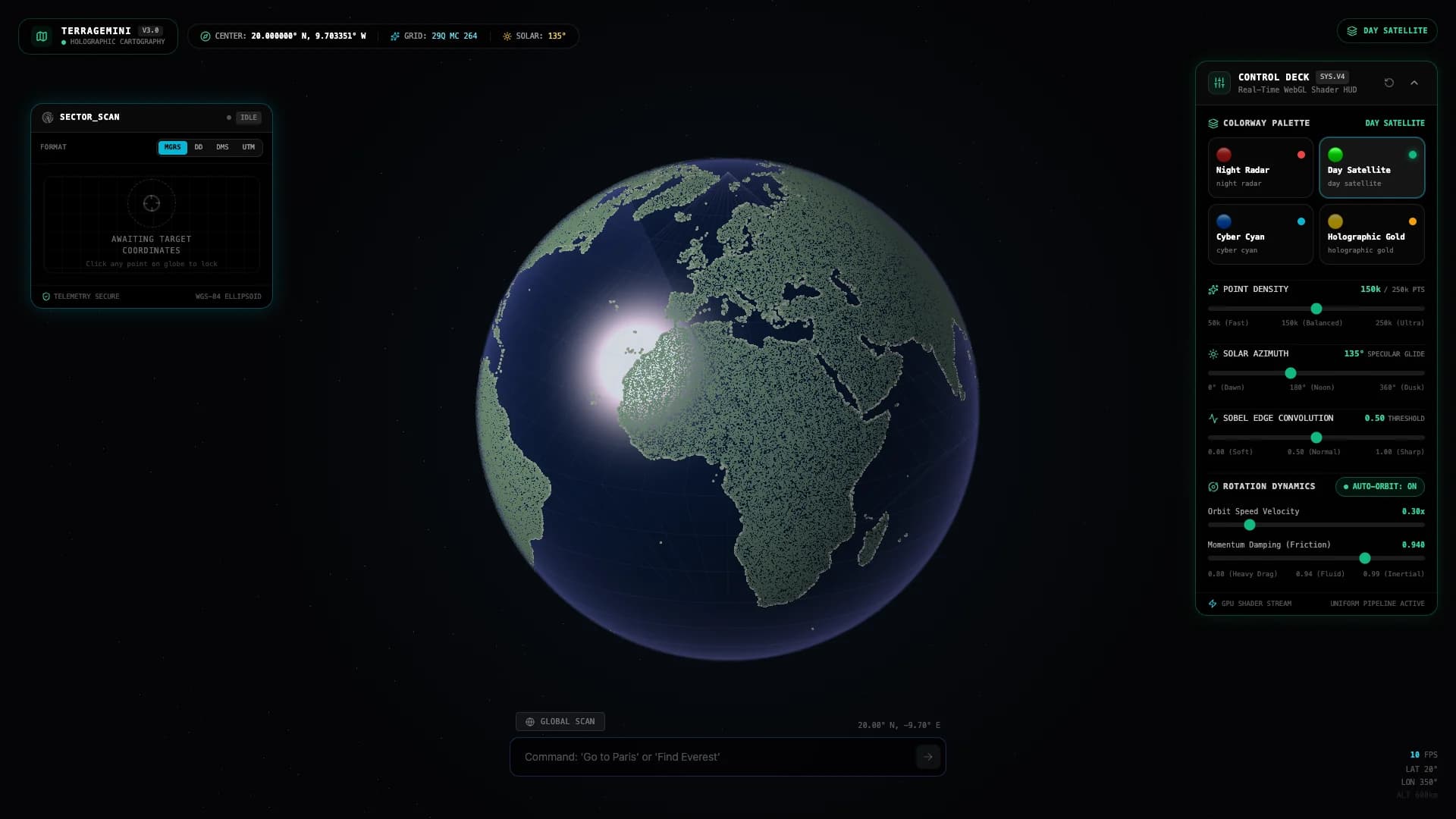
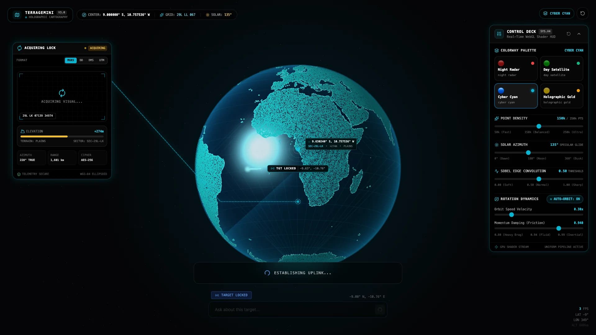
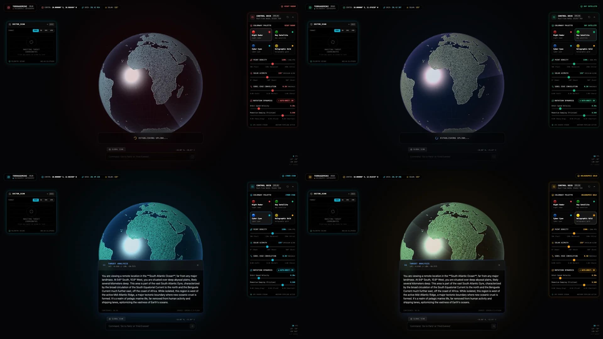
Most AI Studio exports lean on Three.js or React Three Fiber for their 3D work. TerraGemini didn't — it shipped 918 lines of raw WebGL with handwritten GLSL fragment shaders that sample a 2K specular map to separate land from ocean, generate 150,000 holographic dots via UV-space density functions, and trace coastlines using a Sobel edge-detection filter. No abstraction layers, no framework wrappers, just gl.bindTexture and math.
The Elevation Sprint: From AI Studio Export to Military-Grade Planetary Telemetry
While the initial rescue pass made the repository clean and deployable, the second sprint elevated TerraGemini into a flagship WebGL showcase:
- GPU Vertex Buffer Slicing: Rather than reallocating memory when scaling point density from 50,000 to 250,000 points, all points are pre-ranked and uploaded to the GPU once. Scrubbing the density slider simply slices the
gl.drawArrays(gl.POINTS, 0, N)draw range with zero PCIe bus traffic. - Raytraced Blinn-Phong Ocean Glint: An analytic spherical normal vector computed on a billboard quad powers Blinn-Phong specular glint with a scrubbable 3D sun position vector and Rayleigh atmospheric rim scattering.
- Discrete Sobel Normal Gradient: Dynamic convolution kernels extract coastline boundaries and modulate point size () to create crisp continental silhouettes.
- WGS84 Geodetic Engine & Raycast Targeting: Full screen-to-sphere unprojection and forward 3D-to-2D projection with MGRS 1-meter military precision coordinates, radar lock rings, and dynamic SVG leader lines.
- Zero-Recompile Colorway Presets: Instant uniform vector lerping across four visual presets (Night Radar, Day Satellite, Cyber Cyan, Holographic Gold) without shader program relinking or dropped frames.
Timeline
Opened up an AI Studio export called TerraGemini expecting a generic Three.js wrapper and found a 918-line hand-rolled WebGL renderer instead. The entire globe runs on custom GLSL shaders without a single Three.js dependency — separate vertex and fragment programs for dot-matrix land masses, graticule lines, a pulsing location beacon, and a background star field. It pulls 50m TopoJSON data from CDN, rasterizes it onto an offscreen 4096×2048 2D canvas, and runs cosine rejection sampling across the pixel data to generate ~150,000 holographic points with uniform sphere density. There is a built-in momentum physics engine for drag rotation, spring dampening on zoom, and smooth RGB lerping between day mode and amber night mode. The reconnaissance turned up the standard AI Studio detritus — a dead import map pointing to aistudiocdn.com, a missing index.css, and a Vite define block baking PLACEHOLDER_API_KEY straight into the 556KB production bundle. But the core rendering math was pristine, compiling clean across 160 npm packages with zero vulnerabilities.
Shipped TerraGemini to GitHub as a clean standalone repo, but not before learning the hard way why you never trust scaffold artifacts over raw source code. The rescue started with a facepalm — an early plan assumed the app was an image uploader because stale audit notes from export time described a different build before anyone read RotatingEarth.tsx. Once grounded in reality, we stripped the AI Studio scaffolding, added @types/d3-geo and @types/topojson-client alongside an env.d.ts reference so npx tsc --noEmit passed clean, and migrated inline styles to Tailwind CSS 3. The architectural fix was in services/gemini.ts: replacing eager SDK initialization with a lazy getAI() guard that verifies VITE_GEMINI_API_KEY on demand, allowing the 3D globe to boot and spin freely with zero credentials. Because headless Chromium renders blank dark rectangles on WebGL canvases, we spun up a GPU-backed DevTools runner to capture Mount Fuji's AI intelligence card, styled satellite wireframe, and a 36-frame 10fps demo GIF (1.7MB). Shipped in two commits with a 1.28-second Vite production build and zero npm audit vulnerabilities.
In planetary particle visualizers, scaling point density dynamically usually incurs a heavy frame penalty — either through CPU-side vertex buffer re-allocations or repetitive gl.bufferData bus uploads.
TerraGemini eliminates this overhead by pre-generating a maximum pool of 250,000 spherical surface points during the initial raster pass. Each point is importance-ranked (evaluating coastline distance and spatial dispersion) and packed into a single static interleaved vertex buffer ([lon, lat, edge_strength, rank], 16 bytes per vertex) uploaded once at startup.
When the user scrubs the point density slider:
- No CPU memory is allocated.
- Zero vertex bytes are transferred across the PCIe bus.
- The WebGL draw loop executes an range slice:
const renderPoints = Math.min(250000, Math.max(50000, Math.floor(targetDensity)));
gl.drawArrays(gl.POINTS, 0, renderPoints);
Visual presets are managed identically: rather than recompiling shaders or modifying preprocessor #ifdef branches, uniform color vectors smoothly lerp toward target presets via exponential decay () on every frame. The result is instant, 60fps responsiveness across the entire density range.
TerraGemini renders oceanic reflection and planetary atmosphere using a raytraced billboard quad covering the screen-space bounding disc of the planet ().
1. Spherical Normal Reconstruction
For any fragment , fragments outside are discarded. The unit normal on the sphere surface is derived analytically:
2. Solar Vector & Half-Angle Glint
With solar azimuth and constant solar elevation , the normalized light vector is constructed. Blinn-Phong specular intensity is calculated using the half-angle vector with an exponent of :
The step function guarantees that the unlit hemisphere receives zero specular highlight.
3. Rayleigh Atmospheric Limb & Composite
Limb scattering produces an atmospheric rim halo. The final composited fragment combines diffuse ocean tone, specular glint, and atmospheric scattering in a single pass:
To highlight continental boundaries and island archipelagos without adding heavy vector geometry, TerraGemini applies a discrete Sobel convolution filter across the 4K raster landmass mask :
The normalized edge magnitude is computed per vertex:
Dynamic Shader Coastline Modulation
In the vertex and fragment shaders, the uniform u_edge_sensitivity dynamically scales point size and brightness along coastlines:
float threshold = 1.0 - (u_edge_sensitivity * 0.85 + 0.08);
float edgeFactor = smoothstep(threshold, 1.0, a_edge_strength);
gl_PointSize = clamp(baseSize * fresnel * (1.0 + 1.6 * edgeFactor * u_edge_sensitivity), 1.0, 64.0);
This emphasizes continental boundaries while preserving smooth, anti-aliased transitions under high-speed globe rotation.
TerraGemini integrates a full WGS84 ellipsoid geodetic conversion engine with real-time screen-to-sphere raycasting and 3D target lock tracking.
1. Screen-to-Sphere Raycasting
When the user clicks or hovers at screen coordinate , the coordinate is unprojected into spherical unit space relative to center and scale :
If , front-hemisphere depth is computed and multiplied by the inverse camera rotation matrix to extract geodetic latitude and longitude .
2. WGS84 to MGRS (1-Meter Precision)
The geodetic coordinates are processed through a UTM projection engine (calculating meridian arc distance and 5th-order series expansions) and mapped to the Military Grid Reference System (MGRS):
- Derives the 6° UTM zone and 8° latitude band.
- Identifies the 100,000m grid square using DoD/NGA row letter offset sets.
- Produces 1-meter precision coordinates (e.g.
18T WL 83959 07350).
The locked target maintains dynamic 3D-to-2D screen tracking, rendering animated radar rings, occlusion culling on back-face rotation, and dynamic SVG leader lines anchored to the telemetry HUD.