GeoGenesis: mathematical projection unfurling and geodesic routing
1,053 lines of Canvas 2D, continuous Pythagorean limb departure unfurling, multi-projection topology mutators (Winkel Tripel & Mollweide), 24-bit RGB country hit-testing, and Haversine SLERP flight arcs.
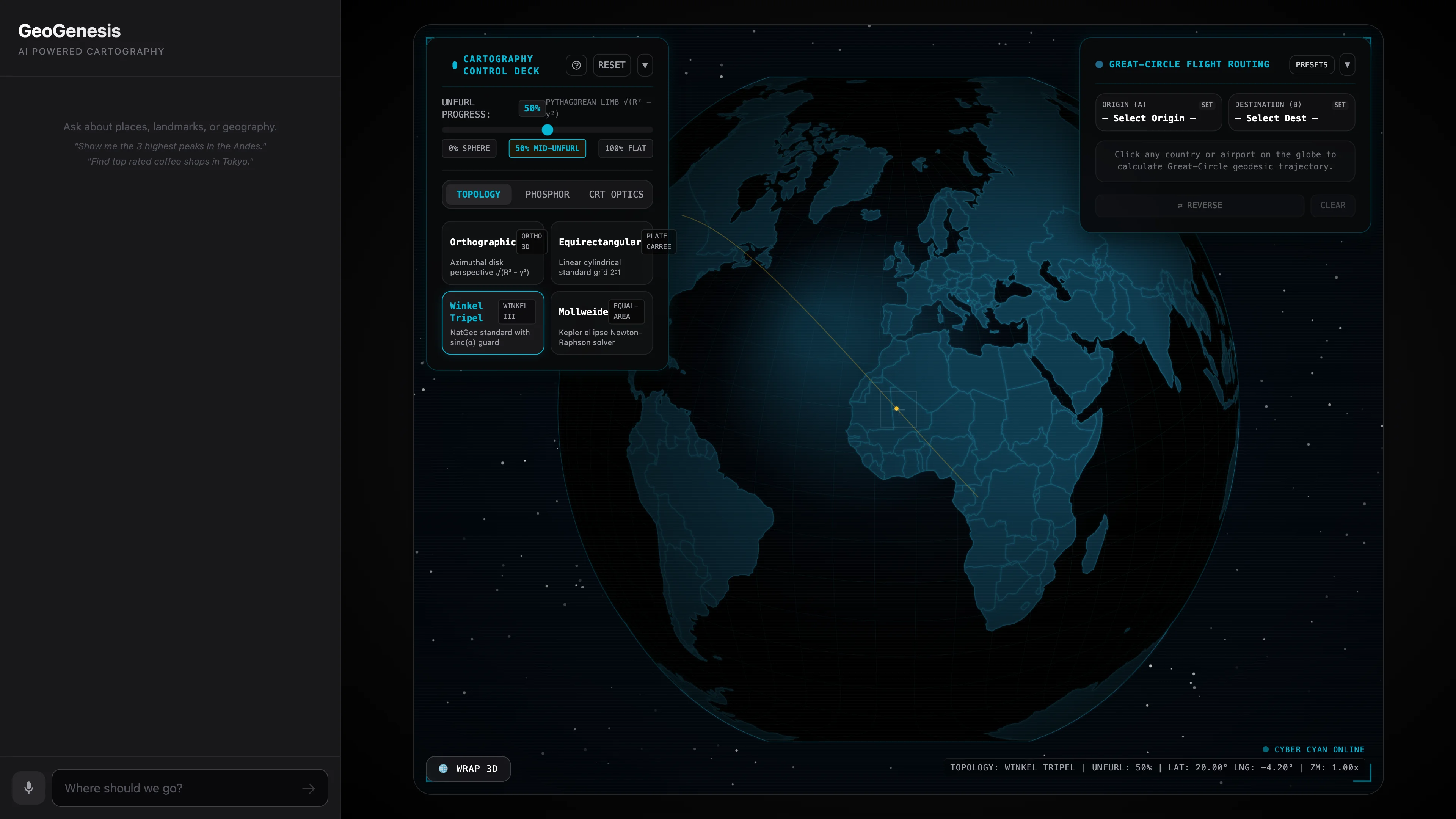
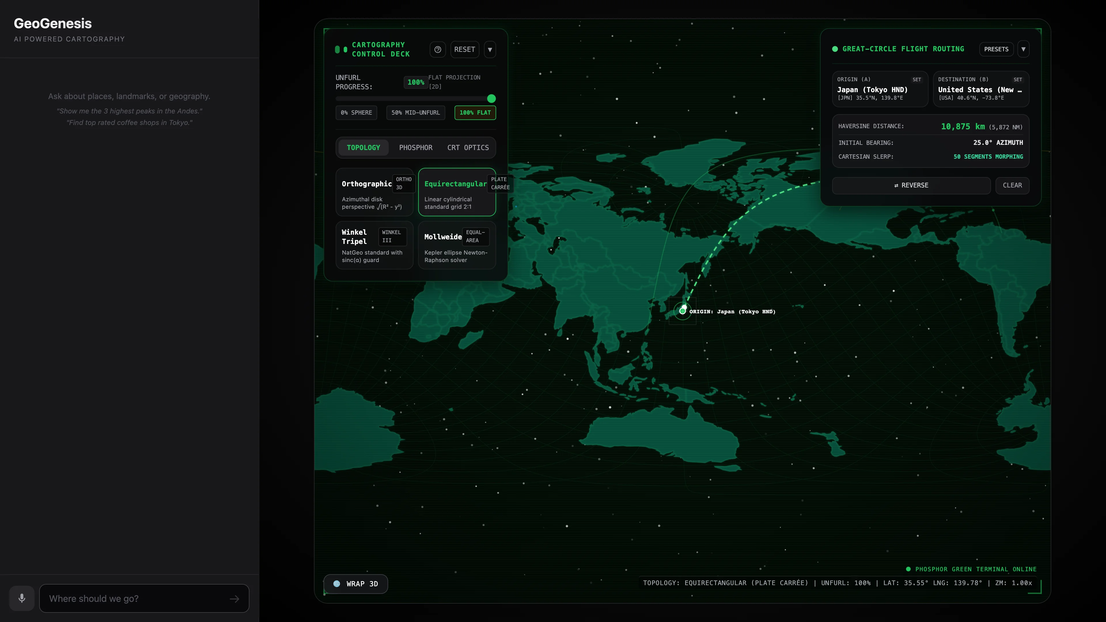
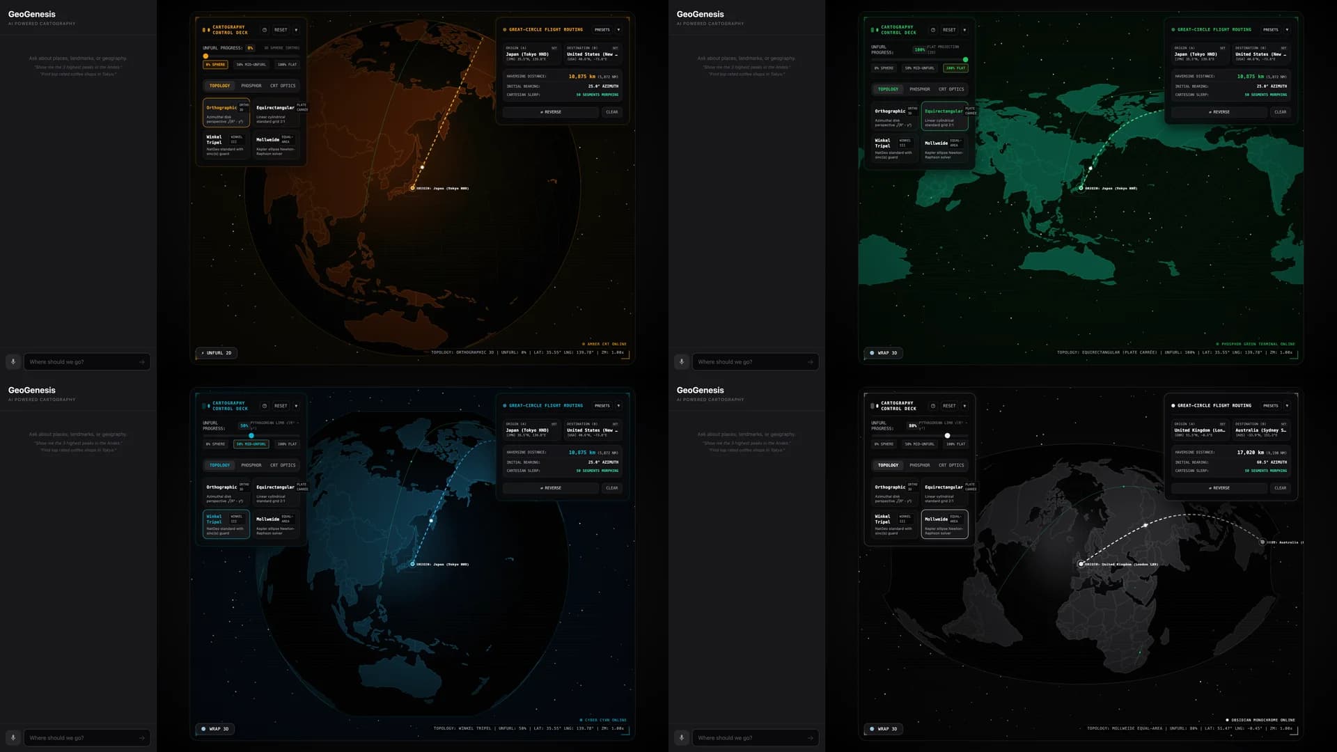
Started with a raw zip file and evolved into an interactive mathematical cartography laboratory.
GeoGenesis arrived as an AI Studio export with a single-file 1,053-line Canvas 2D render loop. The initial rescue repaired Tailwind utility conflicts, patched TypeScript declarations, and verified that the canvas engine delivered 60fps rendering without requiring WebGL or Three.js abstractions.
The Elevation Sprint: Mathematical Rigor & Interactive Projection Lab
The second engineering pass elevated GeoGenesis from a visual demo into a full projection laboratory:
- Continuous Pythagorean Limb Unfurler: Rather than relying on simple cross-fades, the projection transition implements the circular chord bound with parallel limb relaxation and a dynamic clipping horizon .
- Multi-Projection Topology Mutators: Added instant switching between Orthographic, Equirectangular, Winkel Tripel (with 4th-order Taylor series sinc singularity guards), and Mollweide equal-area (solved via quadratic Newton-Raphson Kepler iteration in steps).
- 24-Bit Bijective RGB Picking Buffer: Replaced CPU-heavy geometric raycasts with an off-screen canvas context pinned to host memory via
{ willReadFrequently: true }, decoding country hover states in constant time. - SLERP Geodesic Flight Paths: Integrated spherical linear interpolation across 64 waypoints for great-circle trajectories that dynamically warp and track across the unfolding surface.
Latest Update
Geodesic arc morphing: spherical SLERP flight paths across dynamic projections
Mon, Aug 31, 2026
Timeline
Dropped into a codebase I'd never seen and mapped every wire in under an hour. Traced every import, every config file, every render path — and hit an export called GeoGenesis: a React+Vite app with D3-powered globe rendering, custom projection interpolation between orthographic and equirectangular, a 1,053-line canvas render loop, off-screen color-picking for country hit detection, and a Gemini chat integration with Google Maps grounding. The initial cleanup had already migrated Tailwind from CDN to npm, but left behind Tailwind v4 classes (bg-radial-gradient) in a v3 project — silent CSS failures nobody would notice unless they read every utility class. Found it, flagged it, confirmed both npm run dev and vite build succeed clean. Verdict after recon: this is a keeper — no surgery needed, just a polish pass.
Four CSS bugs hiding in plain sight — all from AI Studio mixing Tailwind versions. The initial cleanup migrated from CDN to npm correctly and pinned Tailwind 3.4.17, but the AI Studio canvas had generated Tailwind v4-only utilities: two bg-radial-gradient calls (main area background and vignette overlay weren't rendering), animate-in fade-in animation classes that don't exist in v3, and a hidden class on the marker tooltip div that would permanently override the JavaScript opacity toggles. Replaced the radial gradients with inline CSS style attributes, swapped the animations for standard Tailwind transitions, removed the stray hidden. The globe went from "nice, but something's off with the depth" to the full CRT-scanline-starfield-vignette atmosphere AI Studio originally intended. Forty minutes from "just get it running" to "it's stunning."
The entire globe lives in a single 1,053-line React component running a requestAnimationFrame canvas loop — no Three.js, no WebGL. GlobeViz.tsx hand-rolls a D3 geoProjection that interpolates between orthographic (sphere) and equirectangular (flat map) using a parameter t from 0 to 1. The projection factory computes per-vertex: x = (1-t) * cosPhi * sinLambda + t * lambda, y = (1-t) * sinPhi + t * phi — a linear blend between Cartesian sphere coordinates and raw lat/lon. Clip angle widens from 90° to 180° as the globe unfolds. Country hit-testing uses a hidden off-screen canvas where each country renders in a unique RGB color from its ISO 3166-1 numeric code — pixel read at mouse position maps directly to country. On top of that: 300 twinkling parallax stars, procedural flight/shipping/data connections animated along great-circle arcs via D3's geoInterpolate, click ripples expanding from coordinates, oscillator-based Web Audio SFX, CRT scanline overlay, corner-bracket HUD, and live telemetry readout. All Canvas 2D.
When transitioning between a 3D orthographic sphere and a planar cylindrical projection, standard GIS frameworks perform hard cuts or opacity fades. GeoGenesis implements a frame-by-frame continuous geometric morpher driven by the Pythagorean limb departure envelope .
1. Parallel Limb Departure Derivation
On an orthographic sphere of radius , surface coordinates map to Cartesian screen coordinates:
At vertical offset , latitude is fixed by . Applying the Pythagorean theorem to the cross-sectional circle parallel to the equatorial plane at height :
2. Continuous Morphing Topology Function
For unfurl parameter (: sphere; : planar projection ), the blended transformation is defined as:
3. Dynamic Horizon Clipping
At , only the visible hemisphere facing the camera is rendered (). As , the clipping boundary expands to reveal the complete planet:
Antimeridian cutting (d3.geoClipAntimeridian) activates when , preventing meridian seam tearing during planar layouts while preserving continuous 3D rotation at .
GeoGenesis supports four cartographic projection topologies: Orthographic (3D disk), Equirectangular (Plate Carrée), Winkel Tripel (National Geographic standard), and Mollweide (equal-area ellipse).
1. Winkel Tripel: 4th-Order Taylor Series Sinc Guard
Winkel Tripel is calculated as the arithmetic mean of the Equirectangular and Aitoff projections, with standard parallel :
At the projection center (), direct evaluation of causes floating-point division by zero. A 4th-order Taylor series expansion eliminates the singularity:
2. Mollweide Equal-Area: Newton-Raphson Kepler Solver
The Mollweide projection requires solving the transcendental Kepler equation for parametric latitude :
Using Newton-Raphson iteration seeded with :
The solver terminates when (typically iterations).
Evaluating point-in-polygon raycasts across 180+ TopoJSON country boundaries during real-time continuous projection morphing causes heavy CPU bottlenecks and dropped frames.
GeoGenesis replaces geometric hit-testing with an off-screen 24-bit bijective RGB color-picking buffer.
1. 24-Bit Bijective Integer Encoding
Each country feature index is mapped to a unique 24-bit integer :
Decoding the pixel value read under the cursor:
If , the pointer is over ocean or void ().
2. Zero-Stall Host Memory Pinning
The off-screen canvas context is initialized with { willReadFrequently: true }. This pins the backing buffer in host memory, eliminating GPU-to-CPU pipeline stalls during ctx.getImageData() calls. Pointer inspection executes in ( constant time) regardless of polygon complexity.
Great-circle paths represent the shortest distance between two points on a spherical surface. As a map morphs between 3D spherical and 2D planar topologies, these trajectories must warp dynamically without distortion or seam breaks.
1. Great-Circle Distance & SLERP Interpolation
Given origin and destination , unit surface vectors are computed. Central angle is obtained via the Haversine equation:
For path parameter sampled across 64 waypoints, spherical linear interpolation (SLERP) generates intermediate surface unit vectors:
2. Continuous Projection Morphing
Each waypoint is transformed through the continuous projection operator:
On the 3D globe (), back-face culling is enforced using camera normal dot products (). Trajectories are rendered with a phosphor glow halo and an animated photon particle with trail decay.